Methods for assessing (fish) abundance - ppt download

Why count? Population size = key demographic/ecological parameter Fisheries (Stock assessment) Conservation & management Research Why would we want to know how many fish there are? … size of the population…. To know the true population size we need to count each and every fish within the population … not realistic Infer ecological processes Age/size structure Trophic structure (energy flow) True population size can be known only if we count each and every individual … not realistic Need to estimate population size based on sampling
Methods for assessing (fish) abundance
Fisheries (Stock assessment) Conservation & management. Research. Why would we want to know how many fish there are … size of the population…. To know the true population size we need to count each and every fish within the population … not realistic. Infer ecological processes. Age/size structure. Trophic structure (energy flow) True population size can be known only if we count each and every individual … not realistic. Need to estimate population size based on sampling.
Based upon… Capture methods. Non-capture methods. Mixed methods. Different methods for assessing abundance. divided into three categories: capture methods, mixed methods and non-capture methods. All have advantages and disadvantages.
Capture methods. Goal. An estimate of relative abundance, based on Catch Per Unit Effort (CPUE) To infer changes in abundance. Unit effort depend of actual mode of capture.
Capture methods I. Seine fishing - net hangs in the water. Trawl fishing (Trawling) net pulled through water or along bottom. Much of the use of CPUE assessment relates to commercial fishing and the estimation of fishing stocks. Which variables define Unit Effort… how many nets of what size and for how long (and how fast) A seine is a large fishing net that hangs in the water by attaching weights along the bottom edge and floats along the top. Trawling is a method of fishing that involves pulling a large fishing net through the water. Long Line fishing (Trolling) – a mainline, rigged with hundreds of short lines (snoods) with hooks, dragged behind a trolling vessel. Pelagic (e.g. for tuna), swordfish; and demersal (halibut) Distinguish Trawl and Troll. Long Line fishing (Trolling) mainline with hanging hooks. Variables that quantify Unit Effort
Other capture techniques are used at smaller scales. Quinaldine, rotenone.
Use of the index relies on two assumptions: Constant catchability (q) Linearity: CPUE = qN. Actual Abundance. Abundance Index : (CPUE) Slope = catchability (q) Providing the assumptions are met, changes in CPUE should be proportional to changes in absolute abundance. The use of the index relies on two assumptions … Why is the linearity assumption important The use of catch per unit effort (CPUE) as a measure of relative fish abundance is a common index used in stock assessment, whether calculated from commercial or recreational fisheries data or from research survey data.
CPUE = qN Linear :  = 1. Non-linear:  ≠ 1. hyperstability - CPUE remaining relatively high while abundance declines. (rate of decline in cpue is smaller than in abundance; at least initially) Hyperdeplition: fish learn to avoid nets. - Hyperstability -  < 1. - Hyperdepletion -  > 1.
Increased catchability (gear effectiveness, skill) Gear saturation (cannot catch more beyond a threshold abundance. Aggregation (effort targeted at areas of high density) As a fish population declines, fish continue to aggregate or school and therefore their local population density remains constant.
(Itai van Rijn) Result were independent of the CPUE index. Does the system suffer from hyperstability
Non-capture methods. Goal. An estimate of the number of individuals per unit area: density. Move on to assessing abundance without capturing. The goal here is usually to obtain an estimate of the density.
The census is carried out within the boundaries of the transect, which is generally denoted out by a flexible graduated tape measure, which is rolled out on the seafloor. Counting is conducted on either side of this tape within a set area. Photo – tape is rolled out during census. No need for earlier deployment which may scare the fish.
One line. (estimate width of transect) Two lines. (deliniated width of transect)
The census is carried out within the boundaries of the transect, which is generally denoted out by a flexible graduated tape measure, which is rolled out on the seafloor. Counting is conducted on either side of this tape within a set area. Photo – tape is rolled out during census. No need for earlier deployment which may scare the fish. More time consuming. Much more information – can be used to remove sampling biases (more about this later …)
(Ori Frid, Ruthy Yahel): Community structure. Groupers per transect.
- Counting while slowly turning around. - Observation for a given period of time. Quicker than laying a transect. Recommended for very heterogeneous environments, and isolated /complex /large structures. Problems: Depends on water visibility. Time adds complexity to analyses. Stationary point. - counting while slowly turning around. - observation for a given period of time. The observer begins counting from a determined point while slowly turning in a circle. This method is quicker than laying a transect. It is particularly recommended for studying a species or small group of species, especially in very heterogeneous environments, and for isolated complex structures or large-size formations (coral heads, large boulders).
Easy to define area. Impossible to simultaneously count fast moving and cryptic species. Usually requires 2-3 passes over the structure: Mobile species counted as in stationary point. Reef associates/ cryptic species counted over a second pass.
Log Area. Does the slope of the species-area relationship change across sites
Can be manned/remote, baited/unbaited. Goal: Indices of relative abundance. Estimates of actual density. Return to Non-capture methods, and look at a slightly different approach. Used in inaccessible environment (deep water) and/or protected areas (non-destructive) Indices: high abundance (shallow water) Estimated densities: low abundances (long time of arrival)
Difficulty obtaining transect area estimate. Advantages: Fast, easy, when done remotely allows access to unreachable regions by diving. Hard copy Disadvantages: Expensive. Requires a lot of processing. Often hard to identify species.
Indices of relative abundance: Maximum number of fish seen in short interval (e.g. 30s; Nmax) Time to peak. Time of first arrival (T1) Models of arrival & departure at the bait, used to infer the actual density. Baited cameras. Often the indices will be correlated, in which case only Nmax is used (number rather than time, although time may be informative in other cases -. E.g if we want to compare the behavior of different species at the bait) There are also attempts to model the arrival and departure of fish at the bait, and to use these models to infer the actual density of fish. (graph: e.g. max N for every 30sec interval)
Estimate species diversity (e.g. species-time curve) Obtain body-size measurements (stereo video) Distance needed to estimate distance. Curve used for comparison (rarefaction) or extrapulation.
Method (belt transect, distance sampling, point count, fixed time) Transect of what size Transect width should match visibility /habitat complexity. Transect length should reflect diving constraints (25m / 50m) What fish to count Impractical to count all fish. Concentrate on certain types of fish: Large/ mobile vs. small/ cryptic. Many times 2-3 passes are conducted over the same transect. Each pass sometimes requires different transect area.
How to divide the work among divers Left/ right vs. far / near. Or. Another replication (how to combine the data )  The division of fish to be counted between divers/ passes is critical! Replications: For advanced statistical methods (occupancy models) several close visitations to the same sites are often needed (to assess detectability)
(Ori Frid, Ruthy Yahel) Distance sampling. 25 m long. Two divers counting simultaneously. (to assess surveyor biases) Only one pass on each transect (cryptic species under-sampled)
Another example of bias, this time – poisoning much more comprehensive coverage of cryptic species and small individuals.
To estimate D … n = no. objects counted. Assumes: Each individual is counted only once. Probability of detection = 1. Problem now is how to estimate P. Probability of detection (P) : probability of detecting an object, given that it is present within a specified area (A) For p<1:
Harder to detect fish further away. Fish escape when divers approach. Fish are attracted to divers. P. x.
To estimate P … Define Detection function , g(x) : Probability of detecting an object, given that it is a distance x away from a transect line or stationary point. w. L. x. For a belt transect with area 2wL. Let’s continue with another definition: detection function. Given this function, we can calculate the detection probability (P), and with that the Density (D). For a belt transect with area 2wL - P and D are given by…
To estimate g(x) … Assume. Objects are uniformly distributed (i.e. Nx = constant) g(0) = 1 (i.e. n0 = Nx) Distance estimated without error. g(x) can be estimated from the frequency distribution of x. The problem now is how to estimate the detection function Remind ourselves that g(x) describes how the proportion of objects which are detected, changes with distance. If we make a couple of simplifying assumptions this relationship can be estimated from the measurements we take during the transect - namely. To estimate the detection function we can use the frequency distribution of the distances at which individuals were observed (how many fish were observed at each distance x_i; n_i). If we assume the distribution of fish is uniform across the sampled area (a constant actual number of fish at each distance i), we are basically looking at a probability of detecting a fish at each distance (n_i / constant). The constant is not known. But if we assume that g(0)=1 then we can calculate actual probabilities (use n_0 as the constant). All we then have to do is fit a function to the distribution of the x’s, integrate it across zer0 to w, and use the integral to solve for D. Number of objects detected at distance x. Number of objects present at distance x.
Mixed methods: mark-recapture. Goal. An estimate of the actual size of a population. [Can also be used to estimate survival and migration rates] Active area of research by biostatisticians that has become very sophisticated. Theory and methods of mark-recapture analysis have been applied to numerous issues in population ecology and conservation; not just to estimate population sizes but also to estimates survival and immigration/emigration rates. We will stick to simple models, aimed at estimating population size; assuming that the population is demographically closed.
Morphological marks. Genetic Marks. To identify fish stock. Mass tagging using chemical or physical markers. Thermal otolith marking.
Physical mutilation (fin clip) Tags: Coded Wire tag. External tags (Petersen discs, Anchor tags) Passive Integrated Transponder tags (PIT) Visible Implant Elastomer tags (VIE)
Issues such as the effect of tagging on survival must be known / examined.
No births, deaths, immigration, or emigration. i.e. total number of individuals is constant during the study. Populations are never truly closed, but they may be practically closed over short periods of time. We’ll consider a simple model applies to what is referred to as demographically closed population. First let’s see what we mean by a closed population.
Two successive surveys (samples) of a population of unknown size (N) 1st survey: A sample of M fish is captured, marked and returned. 2nd survey: Sample of C fish are caught, of which R are marked (recaptured) N= The model is called the Lincoln_Petersen model after… fish populations (Petersen, 1896) and waterfowl (Lincoln, 1930) The model involves two successive samples of the a population of unknown size. 1st survey. M.  N= 2nd survey. C. R.
To the extent that the proportion of marked fish in the population equals the proportion of marked fish in 2nd sample. ≈ M. N. R. C.  Assumptions. All animals are equally likely to be captured in each survey. Capture and marking do not affect catchability. Each survey is random. Marks are not lost between surveys. If we assume that the marked proportion in the sample (obtained in the 2nd survey) is equal to the proportion of marked individuals in the population.
1st survey. M=4. 2nd survey. C=6. R=2. N= Closed population.
- What proportion of the new recruits is spawned locally What proportion of the new recruits is spawned locally
M = Marked output. C = Captured input (total) R = Recaptured (marked input) q. 1-q. R=15. C=5000. R /C = (M/N)  q. Used fluorescent dye to label otoliths of ~106 larvae (eggs from 2000 nests = 0.5-2% of reproductive output) 15 of 5000 sampled pre-settlement juveniles had signs of dye. Pomacentrus amboinensis. A proportion q with have a proportion M/N of marked larvae. M=106. N=5x107 – 2x108. q = 15% (N=5x107) 60% (N=2x108) Jones et al
2nd survey. N= Talking about biases – a few words about sampling, estimation and inference. Let say we did a mark recapture survey and estimated the population size to be 1053 – what can we say about the true population size Not much; unless we also know something about how accurate the estimate is. Not much; unless we also know something about how accurate the estimate is.
The quality of the estimate is linked to its precision & bias. Unbiased & Precise. Unbiased & Variable. Biased & Precise. Biased & Variable. A survey produces a sample statistic (estimate), which is used to estimate a population parameter. Its quality will depend on it bias and precision. To see what each of these mean we need to remember that if we were to repeat a survey many times we would get a different estimate with each replication – the arrows in the picture, which aim to hit the bull s-eye=parameter. We can visualize before we consider an formal definition… The precision of the estimate (how variable are replicated estimates) is a function of sample size . {The variability among statistics from different samples is called sampling error. The standard deviation of the estimate is called the standard error} If the different estimates consistently over/under-estimate the parameter they we would say that it is biased. There are different kinds of bias. (Formally - Bias is the difference between the parameter and the expected value of the statistic) If the statistic is unbiased, the average of all the statistics from all possible samples will equal the true population parameter; even though any individual statistic may differ from the population parameter. The variability among statistics from different samples is called sampling error. Increasing the sample size tends to reduce the sampling error; that is, it makes the sample statistic less variable. However, increasing sample size does not affect survey bias. A large sample size cannot correct for the methodological problems (undercoverage, nonresponse bias, etc.) that produce survey bias. Precision (repeatability): the similarity between estimates. quantified by the standard error Bias / Accuracy: the ‘closeness’ of a statistic to the parameter.
Sampling bias: unrepresentative (non-random) sampling. Estimation bias: due to lower sampling probability of rare values  sample-size dependent. Sample size independent. } Measurement bias – skill of surveyor/operator. Sampling bias - certain age (size) groups / species are scared-off by divers. (appropriateness of a given sampling method) - due to environmental heterogeneity (e.g. habitat complexity, illuminations) . ’’. Therefore, bias leads to an under- or overestimate of the true value. (some people equate accuracy and bias). Bias can arise for different reasons. Measurement & sampling – can not be corrected by increasing sample size. Estimation bias: In a random sample taken from a randomly distributed population, every person in the population has an equal chance of being selected. However, every score in the population does not have an equal chance of being selected. In a randomly distributed population, extreme scores have a lower probability of being selected. Extreme score will tend to be underrepresented in the random sample; causing underestimation (for the variance, correction is by dividing the sum-of-squares by N-1).
… is biased at low sample sizes (small R) Correction for bias: If sample size is small, the above estimator is biased. For example, what happens if the number of recaptures is zero A modified version with less bias was originally developed by Chapman (1951) and is commonly called the modified Petersen estimate in fisheries: Note that Ricker (1975) and many other texts simply drop the -1 as negligible.
Given x mark-recapture studies of same population: As a reminder, the approximate standard deviate of the mean of a sample is mean/sd. For distance based estimates- the variance will depend on the distribution of the distances (g(x)) An approximation based on a single study:
It is impossible to have a method that is unbiased for all species - fish differ in behavior and detection probability. Requires species-specific corrections.  Seldom done (data and time intensive) However, even simple methods are useful for comparing relative abundance across time/space.
Counting fish is like counting trees, except that they are invisible and they keep moving. John Sheppard
There are obvious differences which reflect the biases of the different methods.
Ecologists like to talk about diversity . But what is diversity and how should quantify it Sample A could be described as being the more diverse as it contains three species to sample B s two. But there is less chance in sample B than in sample A that two randomly chosen individuals will be of the same species. Sample A: contains three species to sample B s two. Sample B: less chance (than in sample A) that two randomly chosen individuals will be of the same species.
Evenness: The extent by which species in the community vary with respect to their abundance. Species diversity: A measure that combines richness and evenness. Some definitions related to diversity. First – richness. Second – evenness. Richness can be used as a measure of diversity, either by itself or in combination with some measure of evenness ; as we shall see . (A has higher richness but b has higher evenness) Many indices of evenness (often some measure of diversity divided by its maximum value; obtained when all species are equally abundant)
Rank abundance curve. Species abundance distribution (SAD) As relative abundance is a component of diversity, let see how it behaves across most ecological communities. If individuals in a community are sampled at random, we would usually find that most species are rare while only a few are common. The reason for this pattern has intrigued ecologists since the mid 19th century; but will not talk about it here. We will just note the uneven distribution, and define relative abundance Relative abundance:
Indices of diversity. Shannon entropy: Gini-Simpson index: There are quite a few measures of diversity. Here are two of the most familiar ones; which factor in relative abundance. Species richness is the most straight forward. D: Simpson concentration.
Shannon entropy: A measure of the uncertainty (entropy) associated with correctly predicting the species of the next individual collected. Entropy in predicting species i: Hi = -log(pi)  H’: weighted mean entropy. Shanon entropy = Shanon-Weaver or Shanon Wiener. Based on information theory. How difficult would it be to predict correctly the species of the next individual collected – i.e. A measure the uncertainty in the outcome of a sampling process. e.g. Log2 : minimum number of yes/no questions (on average) Usually uses the natural logarithm (ln). Hmax= log(S), when specie are equally common (max. uncertainty) Hmin = 0, when p of a single species approaches 1 (min. uncertainty)
Gini-Simpson index: The probability that two sampled individuals belong to different species. Gmax= 1-1/S, when specie are equally common. Gmin = 0, when p of a single species approaches 1. Gini-Simpson: Often recommended as a measure of diversity. The sum of all pi’s squared is the probability that two sampled individuals will belong to same species. 1-D: The probability of two sampled individuals belong to different species. As the value of S equally abundant species increases G approaches 1. When the relative abundance of a single species approaches 1, G approaches 0 no matter the value of S. pi: relative abundance of species i. Probability that a randomly picked individual belongs to species i. pi2: probability of two randomly picked individuals belonging to species i.
Measures of diversity. Shannon entropy : information content. Gini-Simpson index: probability. …while these indices are good descriptors of structural complexity, are they good measures of species diversity Of the two most common measures of diversity –one is a probability and the other the information content . While they are good descriptors of structural complexity, are they good measures of species diversity. Let’s look at an example.
Given g(x) we can then formulate an equation for the estimated density. R is the max radius. We will return to this towards the end. R = max. radius.
Studies that compare CPUE data and independent abundance data (research trawl data, used for independent estimations)
Overestimation of abundance. Underestimation of population decline. True pattern. Assumed pattern. CPUE. Assuming linearity - hyperstability can lead to overestimation of biomass and underestimation of fishing mortality. Red : t1. Yellow: t2. Abundance.
quantified by the standard error Bias / Accuracy: the ‘closeness’ of a statistic to the parameter. A survey produces a sample statistic (estimate), which is used to estimate a population parameter. Its accuracy will depend on it bias and precision. To see what each of these mean we need to remember that if we were to repeat a survey many times we would get a different estimate with each replication – the arrows in the picture, which aim to hit the bull s-eye=parameter. The precision of the estimate (how variable are replicated estimates) is a function of sample size . {The variability among statistics from different samples is called sampling error. The standard deviation of the estimate is called the standard error} If the different estimates consistently over/under-estimate the parameter they we would say that it is biased. There are different kinds of bias. (Formally - Bias is the difference between the parameter and the expected value of the statistic) If the statistic is unbiased, the average of all the statistics from all possible samples will equal the true population parameter; even though any individual statistic may differ from the population parameter. The variability among statistics from different samples is called sampling error. Increasing the sample size tends to reduce the sampling error; that is, it makes the sample statistic less variable. However, increasing sample size does not affect survey bias. A large sample size cannot correct for the methodological problems (undercoverage, nonresponse bias, etc.) that produce survey bias. The precision of the estimate (how variable are replicated estimates) is a function of sample size. The bias of the estimate is the extent by which it consistently (i.e. across samples) underestimates or overestimates the parameter. .

PPT - Fisheries Models: Methods, Data Requirements, Environmental Linkages PowerPoint Presentation - ID:5127632

Fish Abundance - an overview

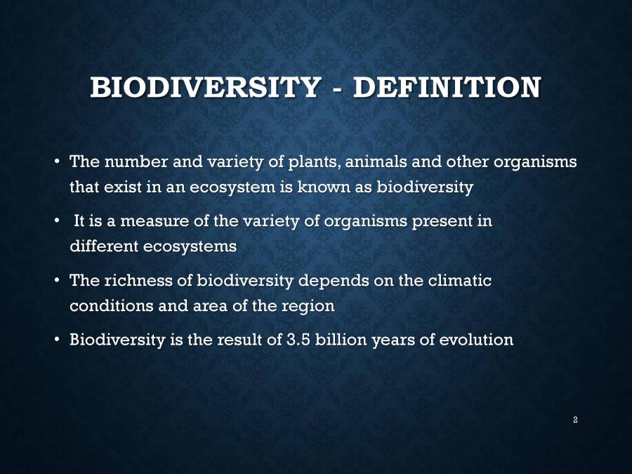
Biodiversity - PowerPoint Slides - LearnPick India

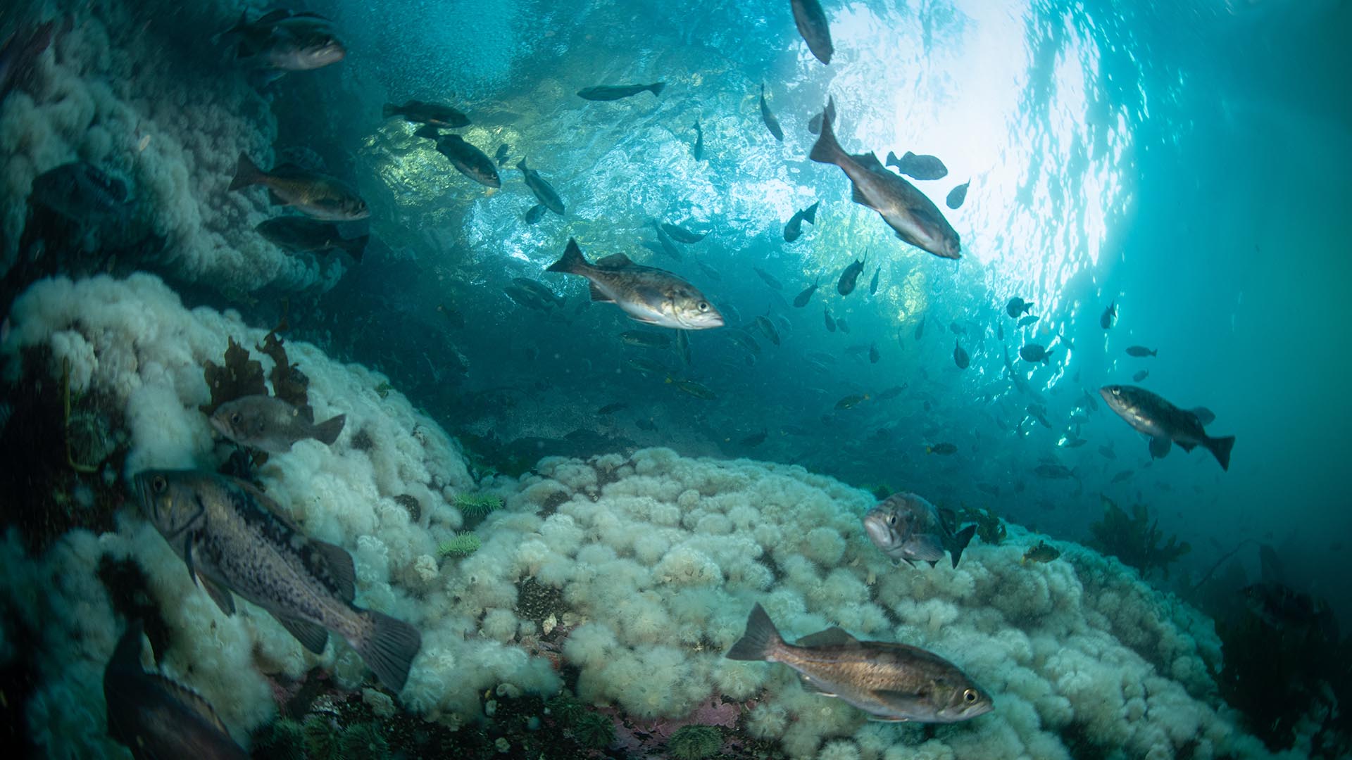
Marine biodiversity Marine Stewardship Council

Palatable Plastics: Assessment of Microplastic Abundance in Pelagic Fish of the Saranac River, NY

Fishing Merit Badge Answers: A ScoutSmarts Guide - ScoutSmarts

Webinar Archive: Sound Production and Reception in Teleost Fishes – Discovery of Sound in the Sea

Metabolic costs associated with seawater acclimation in a euryhaline teleost, the fourspine stickleback (Apeltes quadracus) - ScienceDirect

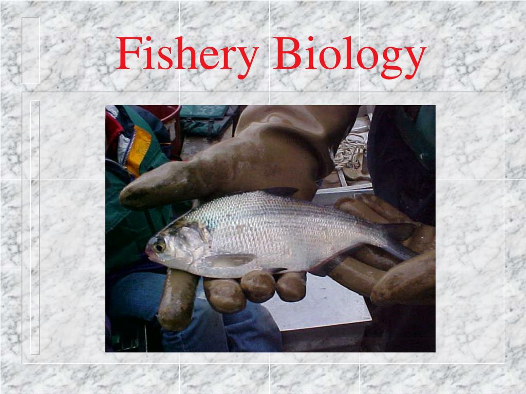
PPT - Fishery Biology PowerPoint Presentation, free download - ID:1031883

Methods for assessing (fish) abundance - ppt download